In my last blog post I wrote about AI-enhancing your existing applications with low risk – and without a huge upfront effort to see if there’d even be value in it for your business. You can just add new AI use cases to your current applications and data, within the database instances that you already have. This approach is possible thanks to all major database vendors now supporting AI vector search and various “AI API calls” in their latest product versions.
Importantly, this means that you do not have to train and even run your own AI models as the hyperscalers do. You can pick a suitable AI model that your cloud vendor offers and let them do all the “question answering” work for you (inference). You’d make your application send some specific bit of information to it as a “question”, often also sending additional context and details to it (RAG) and get back some useful result. Depending on the model and the use case, the input can be a human-written question from some chatbot or just a photo of a customer taken at an automated grocery store.
The output can be a text reply for humans or just an “AI fingerprint” of some detected customer in a vector format, that you can then use with your existing apps. This is where the topic of this post, vector search and using AI in modern databases, comes in.
Index
- What do the new AI use cases mean for databases?
- Data access & I/O patterns of AI vector search in databases
- Stress testing existing workloads and vector search concurrently with Postgres on the Silk Platform
- OLTP transaction and vector search throughput with small I/Os
- Pagecache writebacks when copying data to another filesystem
- Summary
What do the new AI use cases mean for databases?
A short summary is here:
- Your database sizes will grow – you would be storing multi-kilobyte vectors in some new or existing tables, in addition to the usual transaction data. Vector indexes themselves are large too, they can be larger than the indexed table itself
- Your database query volumes will grow – your new AI agent or chatbot might start querying your database for “RAG” (retrieval-augmented generation) to retrieve specific, real-life information about things like your latest product pricing or stock inventory. Caching may help here, unless you need real-time information to avoid mistakes, like overbooking things
- Your database I/O needs will increase – as vector index-based similarity searches are not like precise B-Tree lookups, but more like wide index range scans that can jump into multiple directions (HNSW index)
For “genAI”, like chatbots, you would send/retrieve relevant information from your databases to the generative AI model and let it come back with a response that you then present to the end user. You’d likely verify, “guardrail” and “ground” the correctness and sanity of the response in an additional step, before sending it back, using records queried from your databases (or caches).
For advanced discovery of patterns and “fuzzy” similarities, that are used in recommendation engines, you would interact with embedding models that accept real life input data and return sophisticated “fingerprints” (embeddings). This fingerprint is physically an array of floating point values (typically multiple kilobytes in size) that you’ll then store in your database and use for vector search and comparison later on.
In this post, I will focus on the vector similarity search-based recommendation engine example, as explained in the previous post.
This gives us a good mix of different workloads and database I/O activity. The Postgres database server will be doing heavy concurrent 8kB random reads, checkpoint writes, vacuum I/O, a steady stream of WAL writes, etc. Also, the purchase ranking precomputation batch job will do large parallel full table scans, hash joins and sorts – so we’ll also have lots of concurrent large sequential reads and bursts of write/read I/Os to temporary files – all happening at the same time.
Data access patterns and I/O profiles of vector search queries
Postgres vector similarity search queries with the most commonly used pgvector HNSW indexes look like wide index range scans from the physical data access perspective.
A traditional Postgres B-Tree scan would do a one-directional “linear walk” though the key-range of interest for each query execution. With a suitable B-Tree index, your query might visit only 25 buffers to produce 20 rows of output. For example, accessing 5 index blocks and up to 20 distinct table blocks to fetch additional needed columns for the matching rows for your query (and to ensure that you’ll get the correct version of a row in the table block). B-Tree walking is quite different from navigating through the multi-layered Hierarchical Navigable Small World (HNSW) index graphs. The HNSW scans end up visiting multiple neighboring graph nodes (and data blocks) in many directions, in order to find where to “settle” with their approximate nearest neighbor search.
Depending on your table and index sizes, a single vector search for just one “best match” for your item of interest can easily cause hundreds of buffer visits and I/Os. This results in increased index sizes, more buffers accessed and bursts of random 8kB I/Os, some cached at the OS level, some not.
Here are two examples from vector similarity search queries from my CatBench vector query testing tool. In the first case, I was looking for just one closest match to a “cat-customer” photo when experimenting with a customer identification or fraud detection use case. My SQL query uses “LIMIT 1” to just find the first, closest match from the list of “known customers”, to verify if the latest purchase is also being done by the same customer:
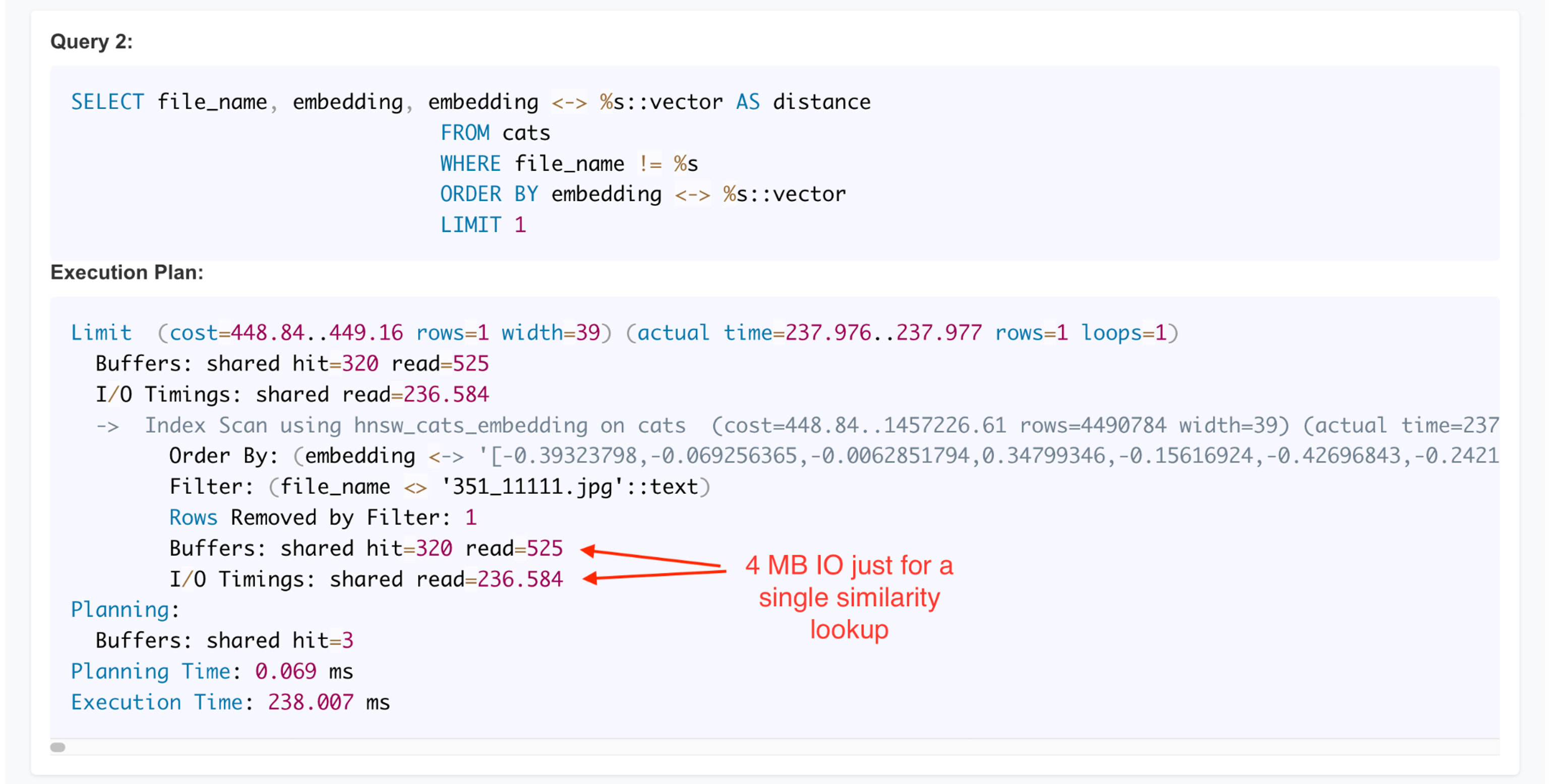
In Postgres plan output, you can add the Buffers: shared hit and read values together to see the total number of block visits. We visited a total 845 blocks, 525 of them did not happen to be in the Postgres buffer cache. So, Postgres had to read 525 blocks from the OS just for this single HNSW-index based approximate nearest neighbor search. As the random reads of 525 different blocks took 236 milliseconds in total, each 8kB pread64()syscall took about 450 microseconds in average. Postgres does not use direct I/O, so all I/Os go through the OS filesystem cache (Linux pagecache in this case), but judging from the Postgres-measured I/O latencies, most of the blocks had to be physically read from the disks. I was running heavy stress tests concurrently on this system, after all.
The second example below uses “LIMIT 20” to retrieve 20 closest neighbors to our (customer) vector of interest. This would be useful for recommendation engines and other clustering or advanced segmentation use cases. This SQL query visited 89 + 905 = 994 buffers. 905 blocks had to be read from the OS! Thanks to the Linux pagecache, some of the blocks were likely read from the OS filesystem cache and didn’t need an actual disk I/O (and/or perhaps I had stopped my other concurrent stress tests by then). This results in a pretty good looking “I/O” latency of 69ms / 905 = 76 microseconds per block read on average.
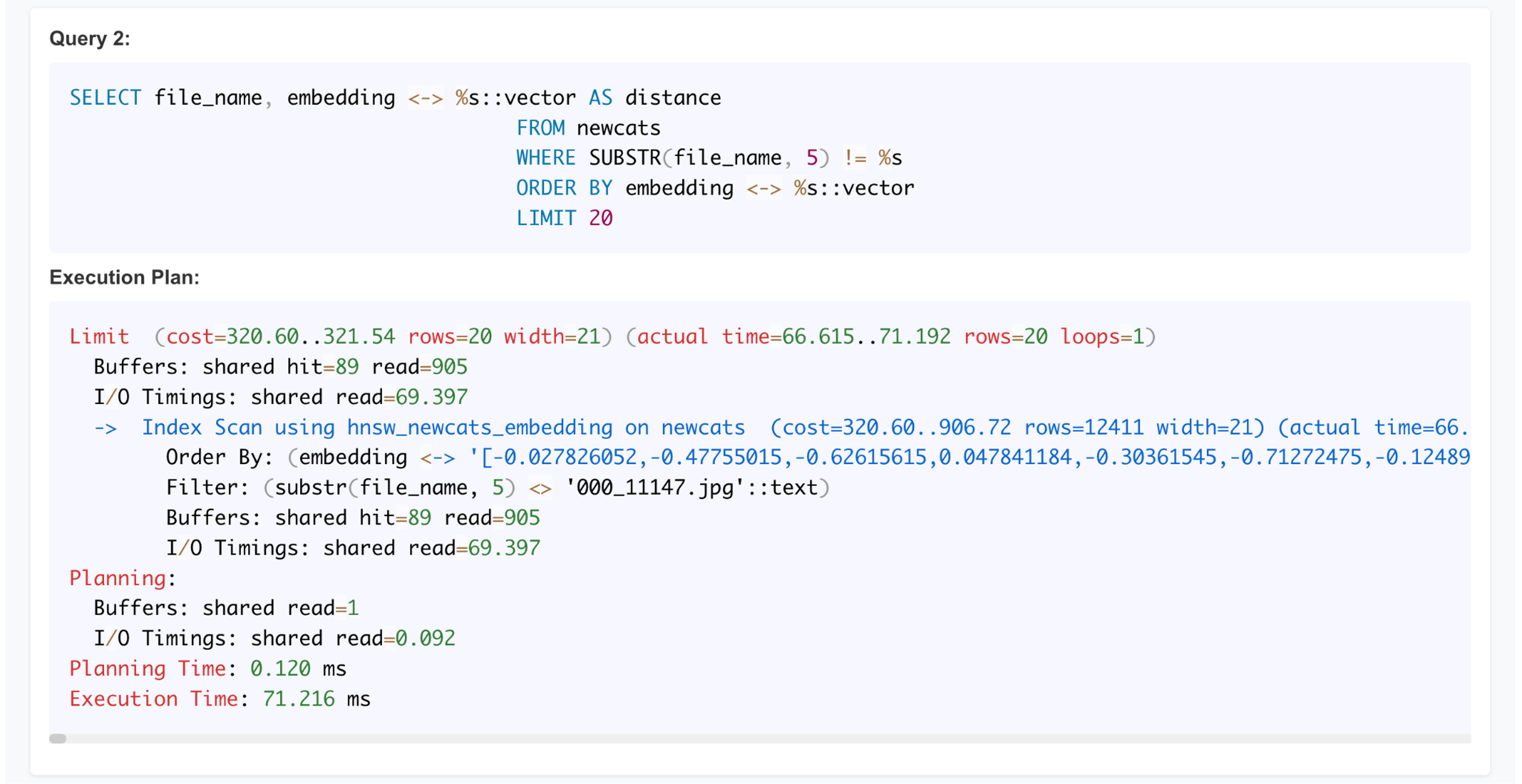
As I said earlier, Postgres pgvector HNSW search queries are like wide index range scans from the data access pattern perspective, they may need to visit hundreds (or thousands) of buffers just to find the 20 nearest neighbors to your vector of interest. As you saw above, reading 500 * 8kB data blocks means 4MB of I/O for a single query!
Now, if you have thousands of online users who are doing similar searches concurrently and expect good response times, both data caching and I/O throughput requirements quickly add up. A bigger server with more RAM for the database buffer cache helps as usual, as does a fast I/O subsystem when it’s not reasonable to try to cache everything in memory.
The search performance of course depends on how big are your tables and a couple of configuration parameters that you can set during the HNSW index creation – but that’s a whole another rabbit-hole and I deliberately left this out of the scope of this post.
Stress Testing Postgres and Vector Search on the Silk Platform
With vector search use cases, you’ll have more data to store in your databases, more data to cache or access. And for best results, you’ll likely have additional batch jobs to summarize and materialize relevant info in new ways – that can then be used in your online, customer facing applications directly. All this activity is what I’ll try to simulate next.
Now we have all the pieces in place for running a stress test with a whole variety of different workloads, all running concurrently:
- HammerDB TPCC stress test – random single block reads, checkpoint writes, WAL writes
- Concurrent random vector index lookups – lots of random single block reads
- Purchase ranking batch job – parallel full table scans, large sequential reads, temp write bursts and reads
This gives us an intense mix of read and write activity – let’s see how the system holds up!
I am not focusing on application code tuning or competitive benchmarking aspects here. I just want to push the entire system throughput as much as possible and see what kind of bottlenecks we might hit at the database, OS and I/O layers. Compared to my Oracle database tests on Silk back in 2021, in this Postgres experiment there are more layers and moving parts involved in the whole system performance. Postgres I/Os go through the OS pagecache and it also uses standard filesystems vs. Oracle that can operate on block devices directly.
I ran these tests on the same Google Cloud VM and Silk setup as shown in my previous post about raw I/O performance testing. I had started my testing on Postgres 16, but Postgres 17 was soon released, so I switched to the latest version instead. I used PgVector v0.7.x then, as v0.8 had not been released yet. The OS was Ubuntu Server 24.04 LTS.
I created a HammerDB TPCC schema with 10000 warehouses, so that the total table/index size on disk was about 1 TB. For example, the customers table had 300M records.
Postgres 17, possibly thanks to its new “streaming I/O” feature, was able to drive physical 5-6 GiB/s of physical read I/O when I just ran a couple of parallel queries that did full table scans through the largest tables, without any additional tuning. Our purchase ranking batch job would run similar parallel scans, but also start writing to tempfiles at some point:
In earlier tests, this single cloud VM was able to deliver over 20 GiB/s of large read I/Os (and separately 1.3M 8kB read IOPS) when tested with fio and without any database or OS pagecache involvement. My parallel queries in this single Postgres database instance were not able to drive this Silk backend anywhere near to its maximum I/O capacity, but sustaining 5-6 GiB/s is still pretty sweet.
In fact, the scanning rate you see above can be handled even with the smallest Silk backend configuration these days, as long as your client-side host VM has enough network throughput allowance in the cloud.
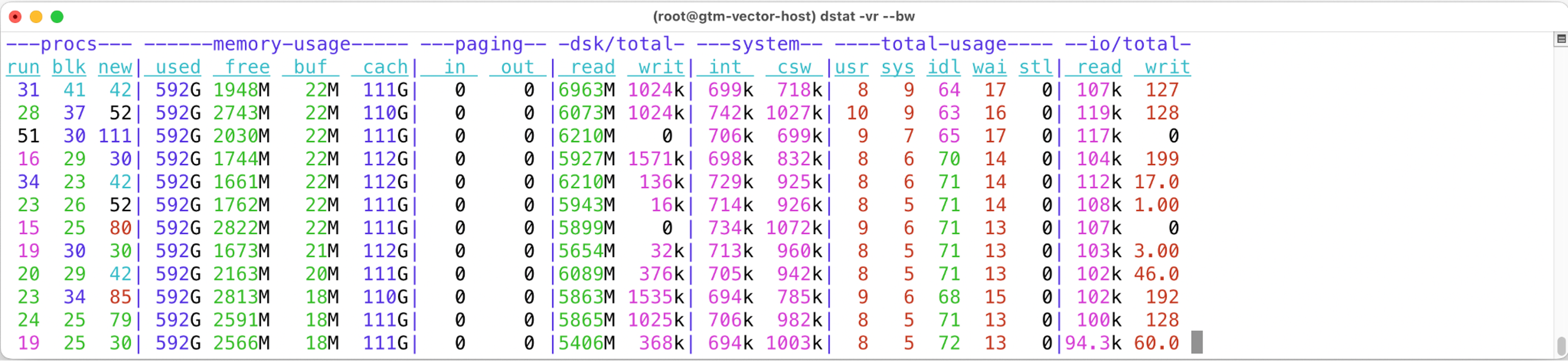
With my parallel queries still running, I then added both the HammerDB TPCC workload and my vector search loops to the mix to generate lots of random 8kB I/Os. Since this cloud VM had 192 vCPUs, I ran HammerDB with 192 clients, plus 4 concurrent loops of my vector search queries that kept running non-stop, without any simulated “user wait time” sleeps:
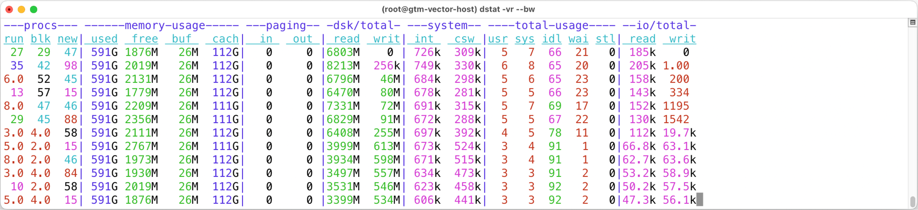
When I kicked the additional stress tests off, I saw a brief jump of both read IOPS and total read I/O rate (up to 8 GiB/s at first), but soon the write I/Os started increasing and the read I/O rate dropped to ~3 GiB/s as you see above. The HammerDB TPC-C benchmark does a lot of table row updates & changes, so it makes sense that WAL writes and checkpoint writes will be added to the mix too. But these are writes, sending data to the storage backend in an opposite direction, so why would reads end up slowing down?
Also, look at the CPU usage figures above, especially the 1st column of dstat (“run”). Why did the number of unblocked, runnable processes drop, despite adding more workload to my stress test?
I avoid guessing if I can, so I measured what all the Postgres processes were spending their time on at the OS level:
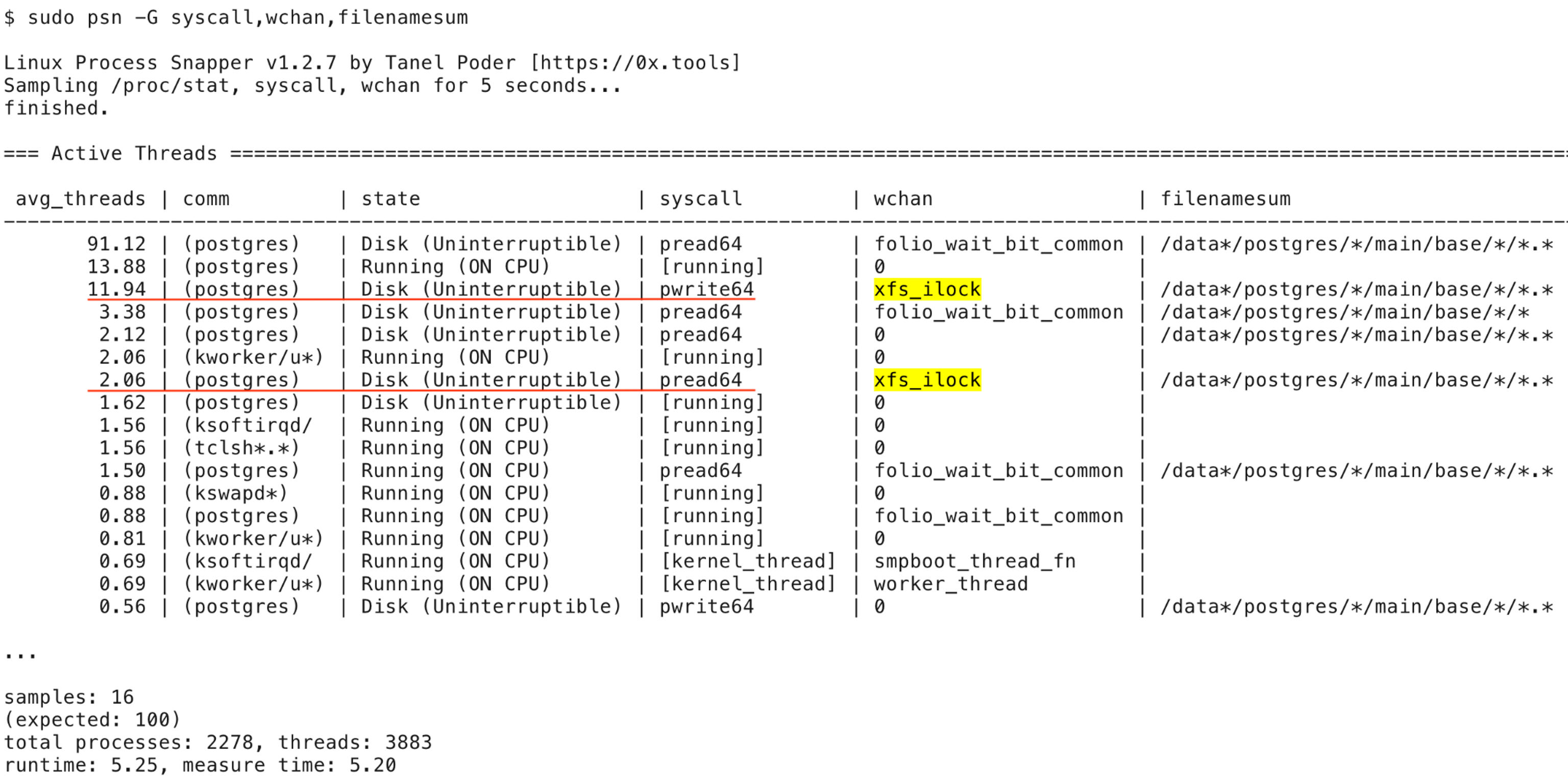
The psn output above shows that while most of the active Postgres processes (91.12 on average) were indeed waiting for their physical I/Os issued via Linux pagecache to complete, there were multiple Postgres processes doing pwrite64system calls too (11.94 reported by psn). These write calls had not reached the actual I/O submission phase in the Linux kernel yet, but were waiting to get an OS file (inode) level lock first. Additionally, a couple of processes underlined above (2.06) were waiting to get the file-level inode lock even before proceeding with their pread64 operation.
This kind of contention is what you get when you mix highly concurrent read and write activity on the same files in Linux. Thanks to the many concurrent write streams introduced by my stress tests, we ended up hitting a Postgres I/O bottleneck at software level (concurrent file access routines in the Linux kernel filesystem layer), not at the OS block device or storage infrastructure level.
Such highly concurrent read/write I/Os are one reason why (for example) Oracle uses its own Automatic Storage Management layer directly on OS block devices, with direct I/O, to avoid any “unnecessary” OS kernel & filesystem-level synchronization bottlenecks.
I’m not complaining about these Postgres results, as I was trying to push just a single large database instance to the max, on a cloud VM with 192 vCPUs and lots of I/O capacity. And I ran multiple different and pretty extreme stress tests concurrently, OLTP transactions, parallel queries and table scans – and vector search loops. In real-life big Postgres databases you’d have many more tables and the largest ones would be partitioned & chunked across many more OS level files, so you’d hit these kinds of bottlenecks much less likely. Especially if you are not trying to fully utilize a 192 vCPU machine!
If you consolidate multiple Postgres databases into one server, they all will operate on their own datafiles, spreading any OS file-level contention over many more objects than in my test.
OLTP transaction and vector search throughput with small I/Os
I also measured the Postgres-reported transaction throughput of HammerDB TPCC stress tests (192 users) and my vector query loops (4 concurrent sessions doing small I/Os), to see what throughput I’d get without having concurrent batch jobs doing parallel reads and writes and this is where I got.
For Postgres monitoring, I used Netdata that’s available as a standard package on Ubuntu 24.04 (or via EPEL on RHEL clones):
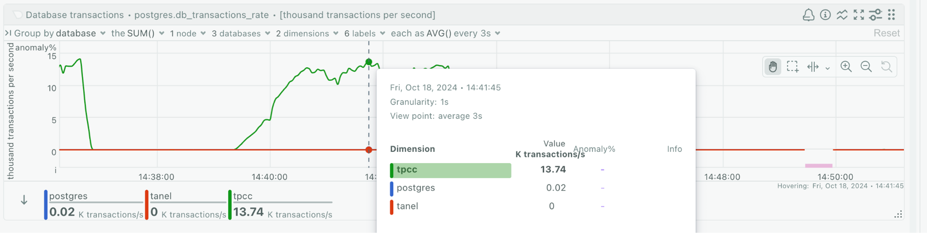
Without the parallel queries in the way, I got to 13k TPCC transactions per second (824k per minute) as you see above. I’m sure there would be application tuning and optimization opportunities here, but this is out of the scope of this article, I just wanted to push the infrastructure as much as possible.
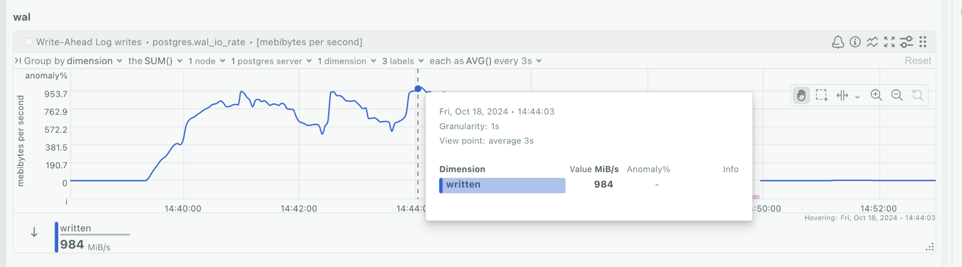
The TPCC workload also modifies lots of records – and the Postgres MVCC approach stores (and later on vacuums) previous versions of entire modified rows – there’s also quite a lot of Postgres WAL/redo-log data generated! Some of my heaviest stress tests consistently generated close to 1 GiB/s of just WAL redo data! The Postgres WAL files are separate from the usual database files, so they don’t end up with a similar OS-level inode contention as described above.
I deliberately placed Postgres WAL logs on a separate filesystem, stored on a separate block device presented by the same Silk backend, so that any WAL I/Os would not get queued up behind regular datafile write bursts at Linux OS block device I/O queue level. Thanks to the Silk platform’s capabilities, these separate “redo” block devices were able to complete their urgent WAL writes (to the same backend) faster than the other concurrent I/Os against the regular datafiles, especially when database checkpoints or other I/O bursts happened.
Pagecache writebacks when copying data to another filesystem
At some point I wanted to test my Postgres workload on a different filesystem setup, so I shut down both the stress test and Postgres database and then used a plain cp command to copy over about 1 TB of Postgres datafiles to another filesystem. The cp command is single threaded and does buffered reads and writes by default, so it will go through filesystem cache, just like Postgres does. It was steadily reading 1-2 GiB/s from the source directory, but its output was first buffered in the Linux pagecache and there was no other I/O going on.
Every now and then the OS pagecache flusher threads kicked in and wrote any “dirty” blocks to the target filesystem’s backing store. It was pretty cool to see how the OS sometimes casually issued 8-9 gigabytes of writes to the Silk block devices every now and then:

This ability to quickly process deep bursts of writes help with database checkpoints and other operations like data loads or SQL parallel sorts and hash joins writing to temp.
Summary
For this article series, I decided to AI-enhance an existing application (HammerDB TPCC) with a vector search use case, all running within the same database schema. It also made sense to include a batch job for pre-computing customer purchase rankings for speeding up the recommendation engine‘s product lookups that would be quickly served online. That allowed me to combine the new customer similarity search feature with already existing transactional data into a single SQL query!
Compared to the raw block I/O results published last year, in this post I added multiple additional layers to my tests. I stress-tested Postgres SQL queries and an application with a mix of workloads using quite different read & write I/O patterns, concurrently. In addition to the Postgres 17 mechanics, we were now dealing with Linux filesystem file access and the OS pagecache effect too.
The Postgres HNSW vector searches look like wide index scans from the database buffer access and I/O profile side, so there was no need to invent new methods to measure an I/O subsystem’s suitability for these queries. We just had to see how far we could push all the random 8kB reads and the general OLTP read/write activity.
Hopefully my last few articles demonstrate that it is possible to AI-enhance your existing applications without huge upfront investments or platform migrations. For best results, you probably need to upgrade some of your existing databases to their latest versions, but that work has to be done at some point anyway. Before committing to production changes, you can easily try out various AI-experiments on your existing data in your (upgraded) development databases, to see which enhancements would bring the best additional value for your business.
It’s also worth looking at outsourcing the entire vector thing to a cloud service (including vector storage) and accessing it all via their APIs, but then you’d lose the ability to use your customer fingerprints as just another table, within your existing application’s schema, with SQL.
Both Postgres and the Silk Platform were able to handle these intense and concurrent workloads, at noteworthy throughput rates. I did not perform any special magic at Postgres level or from the OS perspective, there was just more data and more data access.
As far as trying to reach the previously seen maximum raw I/O testing results (individually: 20 GiB/s large reads, 10 GiB/s sustained writes, 1.3M 8k random read IOPS), in this experiment we hit a software bottleneck first, without ever reaching a “hardware” one. For example, even the smallest Silk configuration can sustain about ~5 GiB/s read rate these days.
Enjoyed this Blog?
Don’t stop now! Deep-dive into AI performance testing by reading the next post in this series. Stay informed and ahead of the curve!
Read the Next Post