Unlock AI Innovation By Boosting Existing Apps with Risk-Free Vector Search

The reason I am excited about the latest genAI and vector search developments is that you can “plug in” these new technologies into your existing applications and their data, without having to re-platform or re-engineer your entire stack first. You can keep your existing application code and database design exactly as it is and then just add new genAI & vector search features where it makes sense.

During the Big Data wave (and hype) 10 years ago, you first had to “find some big data” and then deploy separate data platforms for it, before having a chance to see if it would even provide any real value to your business. Today you can just go through your already existing applications and quickly experiment & validate if there’d be value in adding “AI improvements” for your existing data and apps.

This is possible thanks to database and cloud vendors having already added various vector similarity search and “AI API call” features into their latest product releases. Now it is possible to try out various AI extensions for your existing applications by just using enhanced SQL syntax and APIs provided by your database engine.

I recently ran some high-performance I/O tests on the Silk Platform in Google Cloud, achieving over 20 GiB/s of I/O rate in a single cloud VM. I focused on pushing the limits of raw block I/O at the OS level, but I’m now writing another article about test results of more complex workloads on the same setup. I ran Postgres 17 and the pgvector extension, with a highly concurrent OLTP, vector query and batch job stress test, to see how well all the pieces work together.

In this “prequel” article, I’ll show an example of how I added a simple recommendation engine use case to the HammerDB TPCC schema and my CatBench application, by combining a cat-image similarity search with the TPCC purchase history schema – using a single SQL query.

Adding a recommendation engine to your existing application with vector search 

As I’m specifically interested in the low-hanging fruits of adding some “AI magic” to existing applications, I created a HammerDB (TPC-C) schema containing the “usual application data” that needs to be processed anyway. Then I added a new table called customer_fingerprints that contains embeddings of cat-customer photos from my earlier CatBench post.

This would enable some of AI-powered use cases in your existing application, for example:

1. A product recommendation engine for a (cat) customer that’s currently browsing your webstore. Thanks to vector indexes, you can add a SQL query with embedding vector similarity search into your app that recommends top products bought by other, similar cats that look like your current customer cat. I just used cat photos as the measure of similarity here, but in real-life apps you can compute vectors (using different models) from other signals like purchase history, etc.
2. An extra signal for fraud detection – again, based on just comparing cat photos. This is a complex topic though, as in fully built out applications, you need many additional signals and low-latency decisions for it to be effective in real time. And you still get back only a probability of the transaction’s legitimacy.

Note that my application queries are pretty simplistic as I’m following the existing TPCC schema structure and not building a fully functional application here. I’m interested in measuring how the database engine, vector indexes and the I/O subsystem behave under heavy concurrent workload. This will tell you how much you can push your production databases later on.

Customer Fingerprints table for customer similarity search

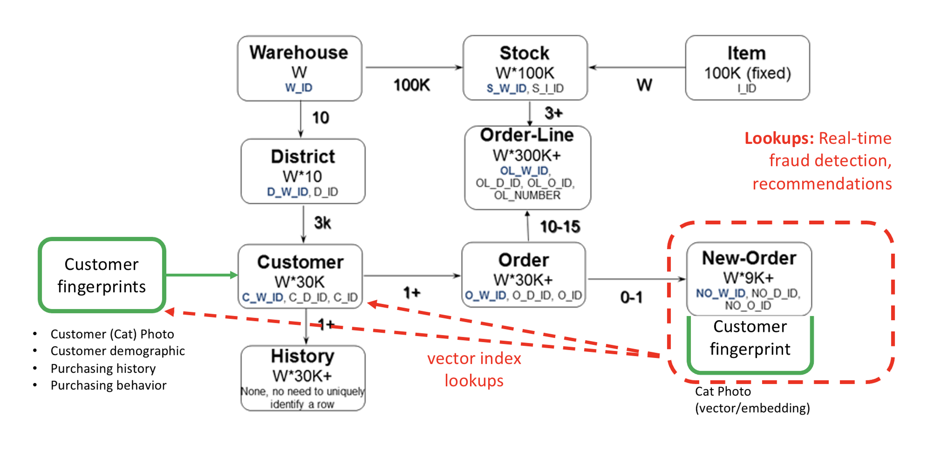
Here’s the HammerDB TPCC schema with the customer_fingerprints table I added, which contains the embedding vector (of a cat photo!) for each TPCC schema customer, so we can later find similar-looking customers for product recommendations:

The new customer_fingerprints table itself looks like this:

tpcc=# \d customer_fingerprints

     Column                      |                                      Type                |

————————–+—————————————-+

 fingerprint_id             |      integer                                             |

 c_id                               |      integer                                             |

 w_id                              |      integer                                             |

 d_id                               |     integer                                             |

 file_name                    |     character varying(100)                 |

 embedding               |     vector(1000)                               |

The file_name field contains the source customer photo and embedding is the vector “fingerprint” that my embedding model returned for this cat photo, to be later used in a similarity search. The c_id, w_id, d_id columns are the ones that allow us to join customer (photo) fingerprints to the rest of the TPCC schema correctly.

To enable vector index-based similarity search, I used the PgVector HNSW type index as it keeps up with subsequent modifications of the table/index data after its creation, unlike the IVFFlat index type. I deliberately left everything to its defaults when creating the index, as at first I’m interested only in the system throughput stress-testing:

SET maintenance_work_mem = ’32GB’;

CREATE INDEX idx_cust_fp ON customer_fingerprints (c_id, w_id, d_id);

CREATE INDEX hnsw_cust_fp_embedding ON customer_fingerprints USING HNSW (embedding vector_l2_ops);

You may want to increase the maintenance_work_mem parameter even further if you have enough RAM, as the HNSW index creation works much faster when it can keep everything that it needs in memory.

Pre-computing ranking for fast recommendation lookups

For recommendation engine’s speed and efficiency, you probably don’t want to run a complex multi-table join to see other similar customers’ top purchases every time a user visits your website, so you can precompute (materialize) the current top favorites of all customers regularly, let’s say once a day. This should be good enough for product recommendations use cases.

For speeding up the real-time product recommendation queries, I pre-computed the top-5 purchased items by each customer (30M customers!) and materialized the results into a customer_top_items table, using the following SQL query.

This customer_top_items precomputation itself did not have to store any vector columns as it’s just a large multi table join and group by operation across existing application tables, to find the exact top-ranked purchases for each customer ID.

The table itself looks like this and I indexed it appropriately for fast lookups during store browsing (just a regular summary table):

tpcc=# \d customer_top_items

                    Table “public.custome

     Column     |         Type          |

—————-+———————–+

 c_id           | integer               | <–

 c_w_id         | integer               | <– composite key (3 columns)

 c_d_id         | smallint              | <–

 i_id           | integer               |

 i_name         | character varying(24) |

 purchase_count | bigint                |

 rank           | bigint                |

This allows me to browse around in the CatBench “customer list” and quickly retrieve vector search-based recommendations that show me the top purchases made by other cats – that visually look like our customer of interest.

Visual walkthrough of the recommendation engine

From the list of customers, I picked one cat and the vector similarity search returned the top 20 most similar-looking ones by navigating through the HNSW index/graph:

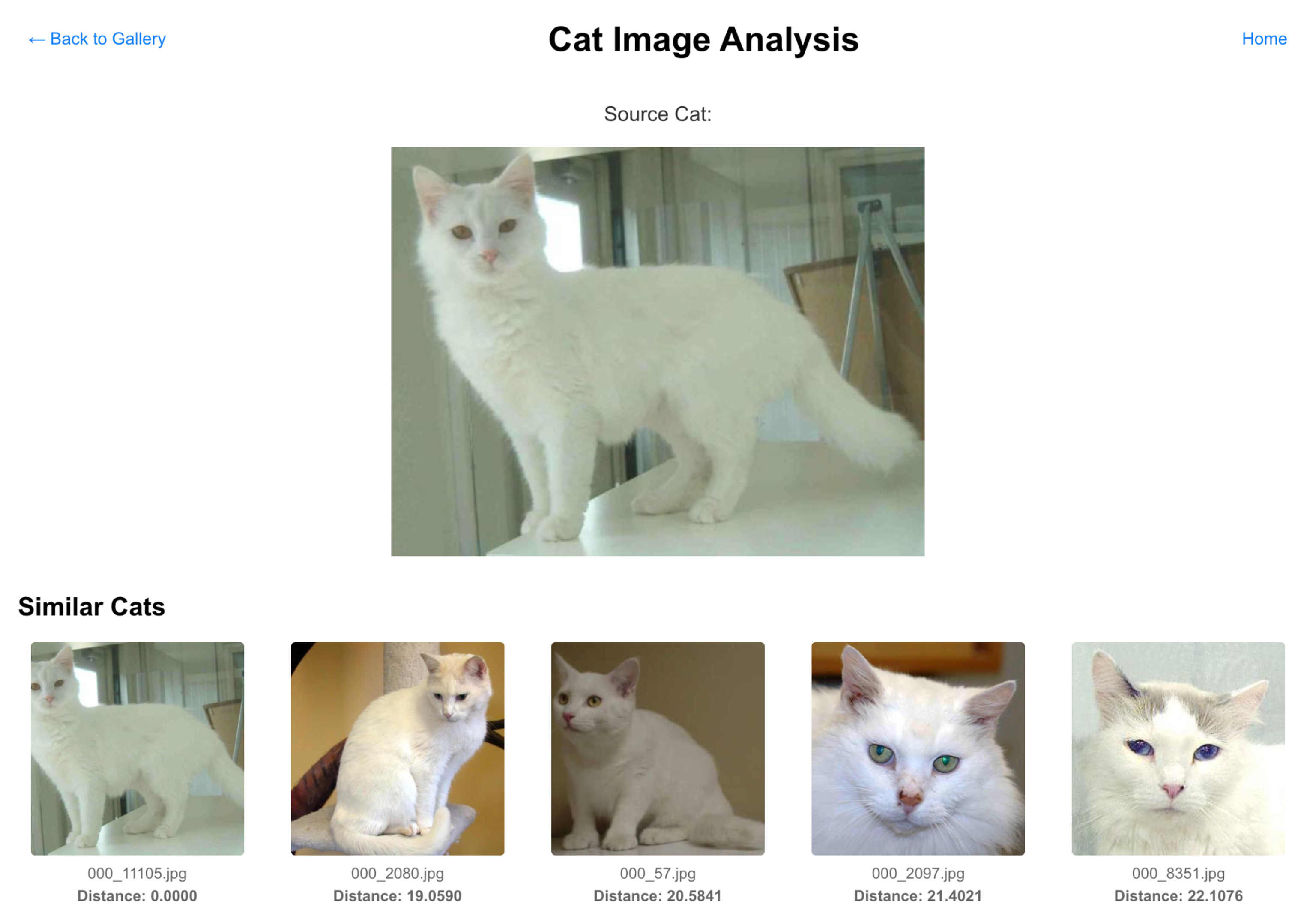
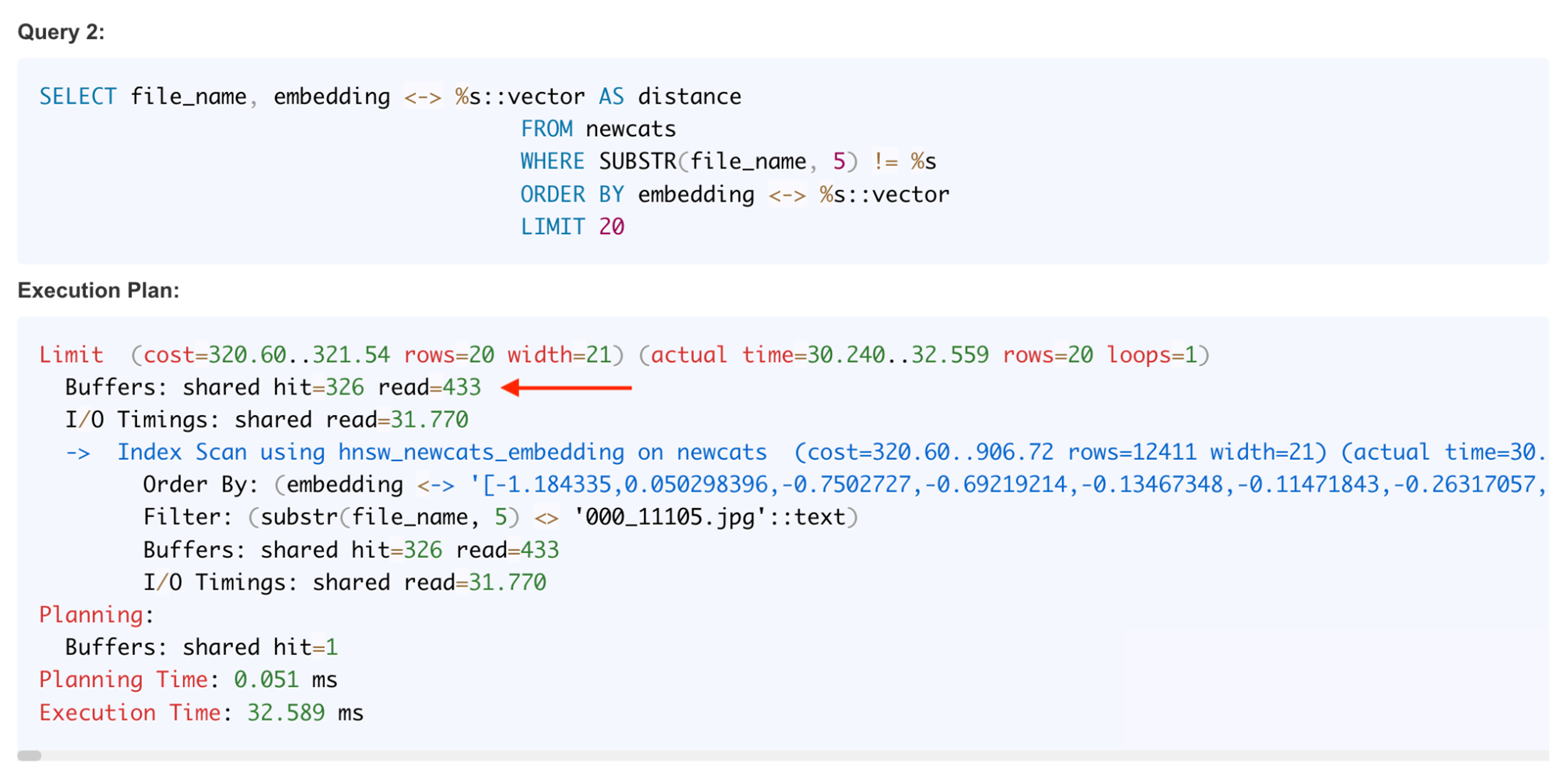
The first matching image above has a distance of 0 – it found the original starting point cat’s picture as the perfect match, I currently don’t filter that out. The query and plan for retrieving 20 closest matches is below. Postgres visited 326 + 433 = 759 data blocks for this search:

The next section below shows popular items purchased by other, most similar customers compared to the chosen cat.

This is where we are blending the traditional application data (order history) with AI-assisted searching of similar customers’ purchases – all executed using a single SQL query within the same database:

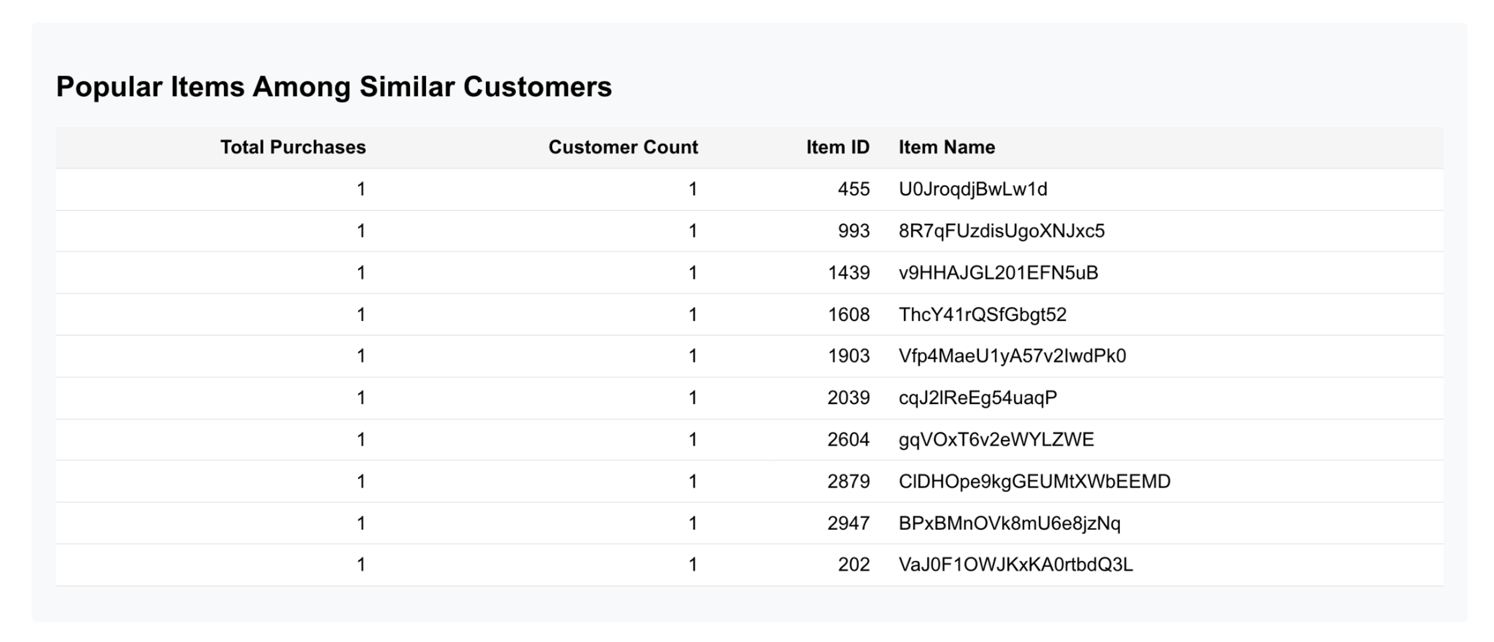
The weird product item names come from how TPCC data generation works, but this is a list of products that other, similar, customers have purchased and it can be used as recommendations to the current customer that’s browsing the online store.

How does it work at the database level? You can combine vector search clauses and regular SQL components into a single SQL statement. Some care is needed as the vector search part should be executed first (driving the whole query execution) and you then feed whatever it returns to the other parts of your query.

This is how I generated the above recommended product list, we start from finding the most similar 20 customers using a HNSW index and then join the results to the rest of the tables in the SQL (using regular joins, no further vector searching needed here):

The execution plan shows a similar flow where we start the query execution from the “Vector index based search” scan on the “hnsw_cust_fp_embedding” index, get 20 closest matches from it and a grand-parent nested loop operation higher up the tree will then use the join keys of these 20 table records to look up top purchases done by the corresponding customers.

To avoid running a complex join 20 times in a loop when generating a real-time recommendation to our webstore customer, I am querying the top purchases from the pre-computed customer_top_items table, with the help of a regular index I had created on it:

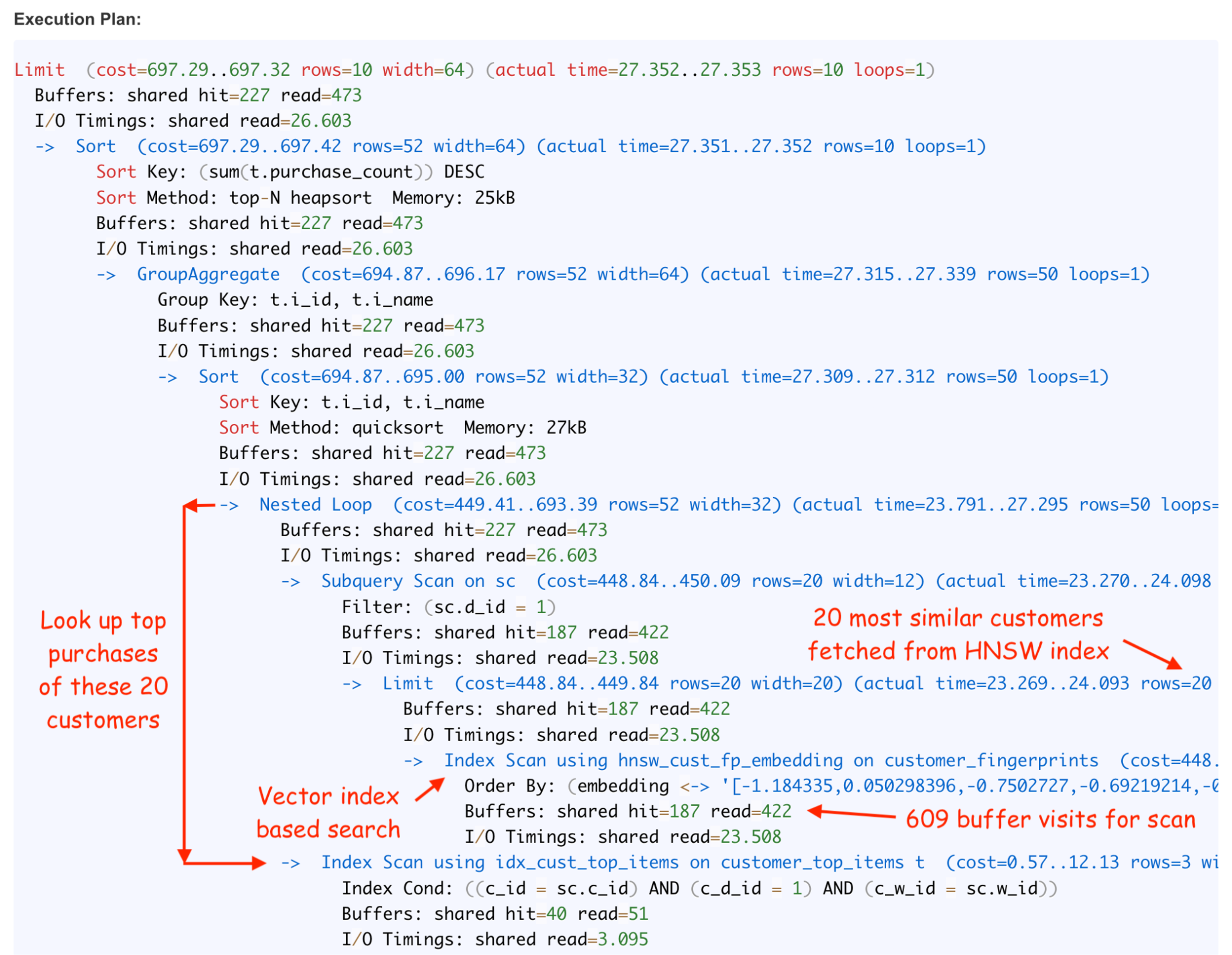
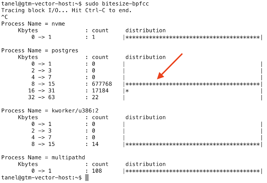
Most of the buffers visited (and physical I/Os issued) by this query were again done at the HNSW vector index access level. That’s just how their navigation works – and it’s all random single block I/Os.

I like to verify these things “physically” on the OS side too and indeed, the bitesize eBPF tool shows that most of the block I/Os done during an HNSW scan are 8kB in size. The few larger ones are likely due to the OS block I/O layer being able to merge multiple I/O requests to consecutive offsets into a single larger I/O:

Customer purchase ranking batch job

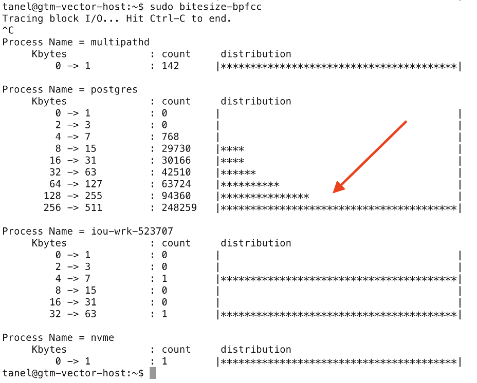
The customer_top_items precomputing batch jobs scans through all customers & orders data using (parallel) full table scans and hash joins, doing multiblock I/Os. Postgres 17 can issue up to 256kB multiblock reads for such scans now – if you set the  io_combine_limit parameter to 32 like I did (the default is 16). Earlier Postgres versions relied on the OS filesystem & pagecache prefetching for large sequential I/Os, but still issued one read syscall for each 8kB block to copy it into Postgres buffer cache.

When I ran some parallel queries with full table scans, I saw plenty of 256kB block I/Os issued, but also plenty of smaller ones too. I didn’t dig deeper, but it’s probably because Postgres is not using direct I/O, so there were occasional “matching” 8kB datafile blocks already cached in the OS pagecache that ended up “breaking” some larger I/O into smaller ones around them.

Actually, after the (parallel) precompute job had been running for a bit, it started doing serious amounts of writes too, as some of the sort and hash areas did not fit into the work_mem allowance. So your reports and analytics doing full table scans across large amounts of data will not only do lots of sequential read I/Os, they may also issue heavy bursts of writes to temp-files too. And that data has to be read back from the temp-files later on as the query makes progress

As businesses look to enhance their applications with AI-driven innovation, vector search is becoming a go-to solution. However, integrating it can introduce challenges like managing vast amounts of data, larger tables, and resource-intensive vector indexes. These factors significantly increase both batch I/O needs and concurrent small I/O demands, putting traditional infrastructure under pressure.

This blog explored how vector search can be seamlessly added to existing applications without risk, enabling AI innovation while maintaining performance and reliability. Stay tuned for the next article, where I’ll demonstrate how these workloads can run concurrently on the Silk Platform for unmatched efficiency and scalability.